SEC | S20W1 | Spreadsheet Essential For Beginners (Spreadsheet Overview, Spreadsheet Interface & Basic Formulas)

Image edited on canva.com
Explain your understanding of Spreadsheet, list its features, its purpose, and the example images that follow your explanation |
|---|
Spreadsheet is a software application that can be used to process various kinds of data, the content in it contains many tables because it does have a function to make various kinds of reports. One of the main advantages of this spreadsheet is because it has a systematic calculation function using various formulas.
When you open a Spreadsheet, you can see that the page only contains small boxes, usually we know it as cells. Each of these boxes can be used to calculate a number of mathematical formulas and various other important data.
I think spreadsheets are also suitable to be used by people who work in data management, accounting and finance. Any amount of data can be processed easily using spreadsheets. The point is, this Spreadsheet itself is very suitable if we want to do various kinds of tasks such as making detailed reports and preparing various kinds of financial plans.
I myself very often use Spreadsheet in my daily activities at school, such as processing student grade data, making attendance reports, making subject rosters and for making all kinds of other documents needed.
There are many similar applications such as spreadsheets as mentioned by the teaching team, but I often use Microsoft Excel if I am in offline mode, if I am in online mode I usually use Spreadsheet from Google.
Spreadsheet features |
|---|
Spreadsheet has many features that are impossible to mention one by one in this opportunity, some of these interesting features I will explain below.
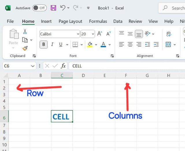
1️⃣ Cells, Rows, and Columns:
Example 1
Cells are the smallest table part in the spreadsheet, here we can add the data and formulas that we need. Rows are horizontal lines that are labeled numerically (1, 2, 3, etc.) You can see them on the left side of the page. Meanwhile, columns are vertical lines that can be identified with letters that are located at the very top of the page.
2️⃣ Functions and Formulas:

Example 2
One of the most used features in Spreadsheet because it has a wide variety of mathematical and statistical functions that can be used for all purposes in analyzing data. Imagine if you have tons of data and have to add them up manually, tiring right?
But with a spreadsheet you only need to add a few formulas and mark which tables need to be summed. All the results will appear by themselves without you needing to sum them manually.
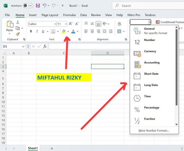
3️⃣ Formatting:
Example 3
Spreadsheets can also be used to format text, numbers, and cells as needed. Such as changing the font, background color, number format, currency format, or date format.
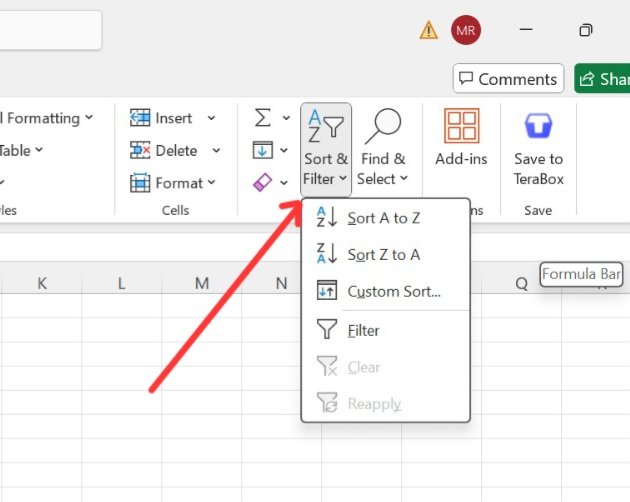
4️⃣ Filter and Sort Data:
Example 4
Analyzing data requires filters and sorting tools, such as we can sort data from largest to smallest or filter only certain relevant data.
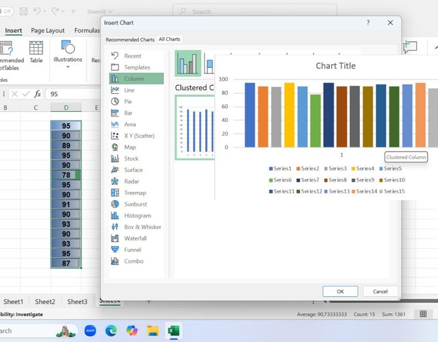
5️⃣ Charts and Diagrams:
Example 5
Another Spreadsheet feature is that we can display data in a visual form such as creating graphs and diagrams, we only need to enter some of the required data and just one click graphs and diagrams are created automatically from existing data. This is very helpful in preparing reports that are more concise and practical.
Based on the basic Formulas given in this lecture, use the data below to calculate the SUM Function and the AVERAGE Function of the class. Show clear working as to how you arrive at your answers. |
|---|
✅ SUM
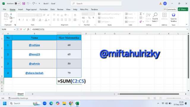
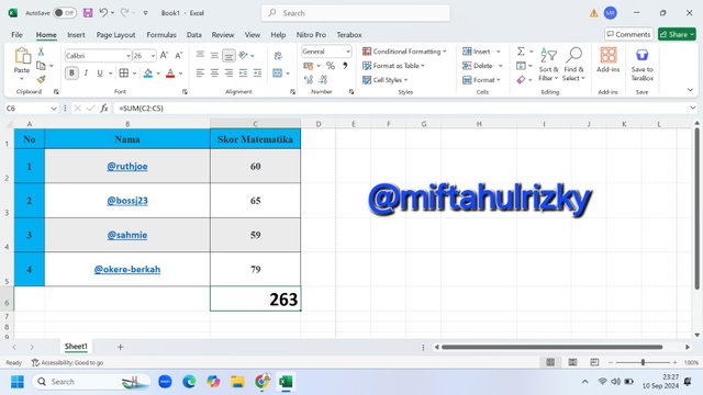
Example of SUM and its results
In this course we have been given four students' data with their math scores, as we can see in the picture that the students' math scores are in column C.
Then we will sum all the scores in columns C2, C3, C4 and C5 using the following formula =SUM(C2:C5) then press the Enter button and the calculation result will come out.
✅ AVERAGE
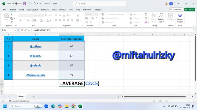
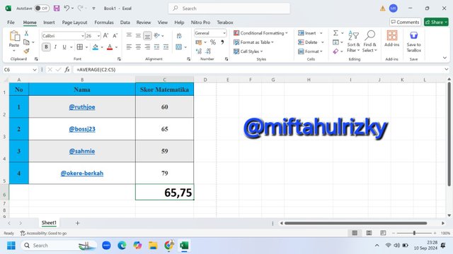
Example of AVERAGE and its results
In this course we are given four student data and their math scores, as we can see in the figure that the student's math score is in column C.
Then we will find the average value of the data displayed in the C2, C3, C4 and C5 columns by using the following formula =AVERAGE(C2:C5) then press the Enter button and the result will come out.
Take a screenshot of your worksheet and identify the cell Addresses of the following; N16 with a fill color of black, J8 with a fill color of yellow B5 with a fill color of Green G12 with a fill color of purple and D1 with a fill color of orange. Write your username on these cells using a visible font. |
|---|
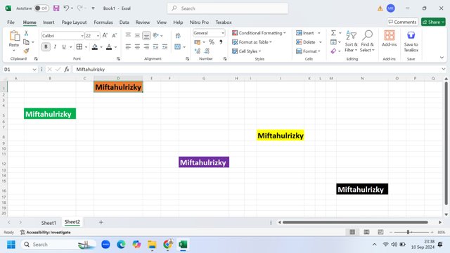
The image above is a screenshot of the worksheet that I have created.
- N16 with black fill color
- J8 with yellow fill color
- B5 with green fill color
- G12 with purple fill color, and
- D1 with orange fill color.
Prepare a score for 15 students where the cell A1 label will be Name, cell B1 label will be Maths Score, cell C1 label will be English Score, cell D1 label will be Physics Score, cell E1 label will be Chemistry Score and cell F1 will be labeled Total. Add all necessary information and calculate the total for each student. Show clear working. |
|---|
As you can see in the image above that we have 15 student data with grades in each subject. The next step we will add up their total grades.Then we will also see how many average grades they get. Besides that, we will also try one of the formulas that can determine whether the student "PASSES" or "FAILS"
🟦 SUM total value

The data used is the data in columns B2, C2, D2, and E2. Then the next step is to write the sum formula =SUM(B2:E2) and then press the Enter button, the result will come out.
🟦 Finding the AVERAGE value
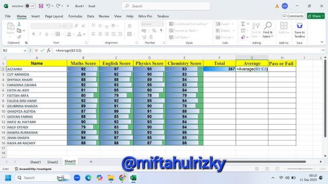
The data used is the data in columns B2, C2, D2, and E2. Then the next step is to write the formula to find the average value =AVERAGE(B2:E2) then press the *Enter" button, then the result will come out.
🟦 PASS or FAIL
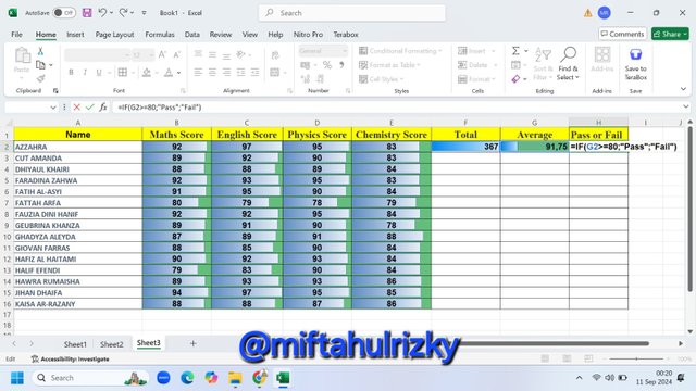
From the picture above, we can see that the average student score is in column G2. To know whether a student passed or not, we must use the following code, =IF(G2>=80;"Pass";"Fail")
If the student's score is higher than 80 then the student is declared PASS, but if the student's score is lower than the predetermined score then the student is declared FAIL.
🟦 Empty column
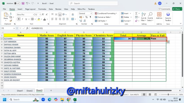

To fill in all the other values can be done in a very easy way, I select the three columns simultaneously in F2, G2, and H2 which in each column has used a number of formulas needed.
The next step is to press the Control button (detained) then pull the cursor down to the required data, then we can see the result that all columns have been filled with the predetermined formulas.

Thus this article, hopefully useful and inspiring all who read it. Thank you for reading this post, don't forget to comment. @kouba01 @irawandedy @fantvwiki
Pemahaman yang bagus dan Penjelasan yang sangat detail, sukses selalu untuk Anda!
Terimakasih sobat, mari berpartisipasi pada tantangan yang sama.
Un gran trabajo el que ha realizado explicando cada una de las fórmulas que ha usado en los cálculos, lo que cual nos hace reconocer la importancia del uso de este tipo de herramientas para digitalizar tareas y obtener cálculos precisos.
Éxitos en su participación.
Those who work every day in processing data certainly need this guideline, thank you for reading this post and leaving meaningful comments.